Hyperion ASO Application level 0 data analysis

In one of my previous blogs I had done some basic analysis on the structure of the BSO Level-0 data extract. Well, now it is time for the data structure analysis of an ASO Essbase application. (I am an ardent ASO fan for some reason. Maybe this has to do with the fact that when I started working in Hyperion initially it was on an ASO application. It was a very cool application and ASO is a bit more technical as compared to BSO, with its tablespaces, bits and stuff.)  

The application that I am going to load data and then analyze the extract is called as ASOSAMP(no surprises there). The structure is as shown in the below snapshot.

I loaded some dummy placeholder data into this application as shown in the below snapshot.

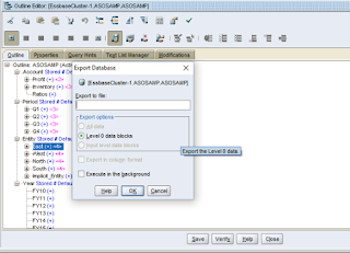
Now, let us start with the export of level 0 data. This is an interesting snapshot.

Now, if you observe the dialog, you will see that for an ASO application, you cannot export data in columnar format nor can you export all level data. This is more of a tradeoff. Traditionally, ASO applications are built for inherently sparse applications, with more than 10 dimensions. If you try to export such a huge data domain of inherently sparse members in columnar format, the file would be enormous and it will be a waste of precious space since the data is the same, formatting is what is taking up the space.

(This is the concept of a tradeoff or as my statistician friends will call, cost benefit analysis. Does doing something actually lead to a benefit or not? If the efforts of doing something outweigh the benefit, there is no point of doing the activity except perhaps as a research curiosity.)

Now the data export is in the format as shown below:-

The ASO data export is very easy to read and in another blog, I plan to actually have a working hypothesis on how the structure is actually derived and how the data is actually stored in the tablespaces. 

This is the nerd talk, you have to pardon me for it. The encoding scheme that is followed for ASO level 0 data is the encoding technique which is technically used for encoding audio files and called as Differential Pulse Code Modulation or DPCM applied to Pulse Code Modulation (PCM). DPCM can be explained as follows from the book Multimedia: Computing, Communications and Applications by Ralf Steinmetz and Klara Nahrstedt.

“It is not necessary to store the whole number of bits of each sample. It is sufficient to represent only the first PCM-coded sample as a whole and all following samples as the difference from the previous one.”

So, the first record in the level 0 export is an entire row with all the dimensions and data represented.

“Sales” -> “Jan” -> “E1” -> “FY16” = 999

 The second line in the extract is Feb=880. This gets interpreted as,

“Sales” -> “Feb” -> “E1” -> “FY16” = 880

The third line in the extract is "Cost of Goods Sold" "Jan" 308. This gets interpreted as follows:-

“Cost of Goods Sold” -> “Jan” -> “E1” -> “FY16” = 308

Thus, at each stage, the current data line is the difference of the members between the previous line and the current line. By only coding what changed between the previous line and the current line, one can have a highly compressed data extract.

Hope you like this analysis of the structure... In one of my next blogs, I will talk about how the export actually happens...Do stay tuned...